What is the relationship between PCB trace width and current?
In PCB design, current-carrying capacity is one of the most misunderstood yet most critical parameters—particularly in power electronics, motor drivers, and high-current control systems. While signal integrity, impedance control, and EMC often receive significant attention, trace current capacity is frequently reduced to rough rules of thumb or “experience-based judgment.” This approach works—until it doesn’t.
Unlike wires, PCB traces are constrained by copper thickness, trace width, thermal dissipation paths, solder coverage, pad geometry, and manufacturing variability.
A trace that appears sufficient under steady-state conditions may catastrophically fail during transient overloads, short circuits, or surge events.
The consequences are often non-linear and destructive, ranging from localized trace burnout to cascading failures across power and signal domains.
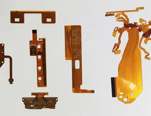
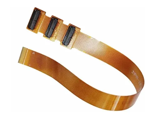
This document consolidates empirical formulas, industry reference data, experimental observations, and hard-earned design lessons related to PCB current-carrying capacity. These empirical formulas are also suitable for Flex PCB and other types of PCB.
It explores the relationships between copper thickness, trace width, temperature rise, solder reinforcement, pad and via geometry, and transient current behavior.
More importantly, it highlights why seemingly minor layout choices—such as pad spoke patterns—can determine whether a design survives a fault condition or self-destructs in microseconds.
Calculation Method:
First, calculate the cross-sectional area of the track. Most PCB copper foil thickness is 35μm (if uncertain, consult the PCB manufacturer; 1 oz = 35μm, though actual thickness is typically less than 35μm).
Multiply this by the line width to obtain the cross-sectional area, ensuring conversion to square millimeters.
An empirical current density value ranges from 15 to 25 amperes per square millimeter.
Multiply this by the cross-sectional area to obtain the current-carrying capacity. I = K × T⁰.⁴⁴A⁰.⁷⁵ (K is the correction factor:
typically 0.024 for copper-clad layers on inner layers and 0.048 for outer layers) T is the maximum temperature rise in degrees Celsius (copper’s melting point is 1060°C) A is the copper-clad cross-sectional area in square mils (Note: square mil, not mm).
I represents the maximum allowable current in amperes (A). Typically, 10 mil = 0.010 inch = 0.254 mm corresponds to 1 A, while 250 mil = 6.35 mm corresponds to 8.3 A.
Data:
Calculating PCB current-carrying capacity has long lacked authoritative technical methods or formulas. Experienced CAD engineers can make relatively accurate judgments based on personal expertise.
However, for CAD novices, this presents a significant challenge. PCB current-carrying capacity depends on the following factors: trace width, trace thickness (copper foil thickness), and allowable temperature rise.
It is widely understood that wider PCB traces carry greater current. Here, consider this: assuming identical conditions, if a 10MIL trace can handle 1A, would a 50MIL trace handle 5A? The answer is clearly no.
Refer to the following data provided by an international authoritative body:
- Unit for trace width: Inch (inch = 25.4 millimeters)
- 1 oz. copper = 35 microns thick, 2 oz. = 70 microns thick
- 1 OZ = 0.035mm
- 1mil. = 10⁻³ inch.
Experiment
Experiments must also account for voltage drops caused by wire resistance due to length. Solder applied during process soldering merely increases current capacity but makes precise volume control difficult. A 1-oz copper wire, 1mm wide, typically handles 1-3 A currents, depending on wire length and voltage drop requirements.
The maximum current rating refers to the permissible value under temperature rise constraints, while the fuse value indicates the current at which the temperature rise reaches copper’s melting point. Eg. 50mil 1oz with a temperature rise of 1060°C (copper’s melting point) corresponds to a current of 22.8A.

Table 1
Relationship Between PCB Copper Thickness, Trace Width, and Current
Before exploring the relationship between PCB copper thickness, trace width, and current, let’s understand the conversion between ounces, inches, and millimeters for PCB copper thickness: “In many datasheets, PCB copper thickness is often specified in ounces. The conversion between ounces, inches, and millimeters is as follows:
- 1 oz = 0.0014 inches = 0.0356 millimeters (mm)
- 2 oz = 0.0028 inches = 0.0712 millimeters (mm)
Ounces are a unit of weight. The conversion to millimeters is possible because PCB copper thickness is measured in ounces per square inch.”

Table 2 PCB Design Copper Thickness, Line Width, and Current Relationship Table.
The current-carrying capacity of a conductor is directly related to the number of vias and pads present on the conductor line (currently, no formula has been found to calculate the impact of pads and via apertures per square millimeter on the line’s current-carrying capacity; interested individuals may research this further, as I am not entirely clear on this and will not elaborate here).
Here, we will briefly outline some primary factors affecting a line’s current-carrying capacity.
1. The current carrying capacity values listed in the table represent maximum values at standard room temperature (25°C). Actual design must account for environmental conditions, manufacturing processes, substrate materials, board quality, and other variables. Therefore, the table provides reference values only.
2. In actual design, each conductor is also affected by pads and vias. For instance, segments with numerous pads will see a significant increase in current-carrying capacity at the pad locations after solder wetting. Many have likely observed sections of trace between pads being burned out on high-current boards.
The reason is straightforward: after solder wetting, the presence of component leads and solder enhances the current-carrying capacity of that segment.
However, the maximum current a pad-to-pad connection can handle is limited by the maximum current the pad width permits.
Consequently, during instantaneous circuit surges, the pad-to-pad segment is prone to burning out. Solutions: Increase the trace width. If the board does not permit widening the trace, add solder layer to the trace (typically, a 1mm trace can accommodate an additional solder layer trace of about 0.6mm; alternatively, you can add a 1mm solder layer trace).
After solder overpass, this 1mm trace can be considered equivalent to a 1.5mm~2mm trace. (Depending on solder distribution uniformity and volume during soldering), as shown below:

Figure 1
Such techniques are familiar to those designing small appliance PCBs. With sufficiently uniform and abundant solder coverage, this 1mm trace can effectively function as a 2mm trace. This aspect is particularly crucial in single-sided high-current boards.
3. The treatment around the pads in the diagram similarly enhances the uniformity of current-carrying capacity between the conductor and the pad.
This is especially important in boards with thick, high-current leads (where the lead width exceeds 1.2mm and the pad diameter is over 3mm).
If a pad exceeds 3mm and the pin exceeds 1.2mm, the current flowing through this pad after soldering increases by several dozen times.
During high-current surges, the current distribution across the entire circuit becomes highly uneven (especially with numerous pads), significantly increasing the risk of burnout between pads.
The approach shown in the diagram effectively distributes the current load across individual pads and surrounding traces, improving uniformity.
Finally, note: Current carrying capacity data sheets provide absolute reference values.
For non-high-current designs, adding 10% to the specified values will fully meet design requirements.
For typical single-sided PCB designs with 35μm copper thickness, a 1:1 design ratio is generally sufficient.
This means a 1mm conductor can handle 1A current while meeting requirements (calculated at 105°C).
Relationship Between PCB Copper Foil Thickness, Trace Width, and Current
Signal Current Intensity. When the average signal current is high, consider the current capacity of the trace width. Trace widths can be referenced from the following data:
Current carrying capacity for copper foils of different thicknesses and widths is shown in the table below:

Table 4 Relationship Between Copper Foil Thickness, Trace Width, and Current in PCB Design
Notes:
i. When using copper foil as conductors for high currents, the current-carrying capacity of the foil width should be selected by derating the table values by 50%.
ii. In PCB design and manufacturing, OZ (ounce) is commonly used as the unit for copper foil thickness. 1 OZ copper thickness is defined as the weight of copper foil per square foot, corresponding to a physical thickness of 35μm; 2OZ copper thickness is 70μm.
Empirical Formula
I = K × T⁰.⁴⁴A⁰.⁷⁵
K is the correction factor, typically 0.024 for copper-clad traces on inner layers and 0.048 for outer layers. T is the maximum temperature rise in degrees Celsius (copper’s melting point is 1060°C).
A is the copper-clad cross-sectional area in square mils (not square millimeters).
I is the maximum allowable current in amperes (A).
Typically, 10 mil = 0.010 inch = 0.254 mm corresponds to 1 A; 250 mil = 6.35 mm corresponds to 8.3 A.
Calculation method provided by a netizen:
First, calculate the track cross-sectional area. Most PCB copper foil thicknesses are 35μm (if uncertain, consult the PCB manufacturer). Multiply this by the line width to obtain the cross-sectional area, ensuring conversion to square millimeters.
An empirical current density value of 15–25 amperes per square millimeter applies. Multiply this by the cross-sectional area to determine the current-carrying capacity.
Insights on Trace Width and Via Fill
When designing PCBs, we generally follow a common practice: use thicker traces (e.g., 50 mil or larger) for high-current paths, and thinner traces (e.g., 10 mil) for low-current signals.
For certain electromechanical control systems, instantaneous currents exceeding 100A may flow through traces. In such cases, narrower traces will inevitably fail.
A fundamental rule of thumb is: 10A/mm². This means a trace with a cross-sectional area of 1 square millimeter can safely carry 10A. If the trace width is too narrow, it will burn out under high current.
Of course, current-induced trace burnout follows the energy formula: Q = I²t. For instance, a trace carrying 10A can withstand a 100A current spike lasting microseconds—a 30mil trace would certainly survive.
(This raises another issue: the trace’s stray inductance. This spike will generate a strong counter-electromotive force due to this inductance, potentially damaging other components. Thinner and longer traces have greater stray inductance, so practical design must also consider trace length comprehensively.)
Most PCB design software offers several options for routing copper pads around component vias:
Right-angle radiating pads, 45-degree radiating pads, and straight pads. What’s the difference? Beginners often overlook this, choosing randomly based on aesthetics.
This is unwise. Two key considerations exist: preventing excessive heat dissipation and ensuring adequate current-carrying capacity.
Using straight pads significantly enhances the pad’s current-carrying capacity. This method is essential for device pins in high-power circuits.
Simultaneously, it offers excellent thermal conductivity. While beneficial for device cooling during operation, this poses challenges for PCB soldering personnel.
The pads dissipate heat too rapidly, making it difficult to hold solder. This often requires higher-wattage soldering irons and elevated soldering temperatures, reducing production efficiency.
Using right-angle or 45-degree radiating pads reduces the contact area between the pin and copper foil, slowing heat dissipation and making soldering much easier.
Therefore, selecting between straight or angled via pads for copper plating should be based on application requirements, balancing both current-carrying capacity and heat dissipation.
Avoid straight plating for low-power signal lines, while high-current pads absolutely require straight plating. Whether to use right-angle or 45-degree pads is primarily an aesthetic choice.
Why bring this up? Because I’ve been troubleshooting a motor driver for some time now. The H-bridge components kept burning out, and for four or five years, I couldn’t pinpoint the cause.
After much effort, I finally discovered: it turned out that during copper plating, the pad for one component in the power circuit used a straight-angle spoke pattern (and due to poor plating execution, only two spokes actually appeared).
This drastically reduced the power circuit’s overcurrent capacity. While the product functioned perfectly under normal 10A operation, a short circuit in the H-bridge would draw around 100A.
These two traces would instantly burn out (within microseconds).
Consequently, the power circuit becomes open-circuited. The energy stored in the motor, lacking a discharge path, dissipates through every possible route.
This energy surges through the shunt resistor and related operational amplifier components, obliterates the bridge control chip, and infiltrates the signal and power lines of the digital circuitry, causing catastrophic damage to the entire device.
The entire sequence unfolds with the same breathtaking intensity as detonating a massive landmine with a single strand of hair.
Conclusion
PCB current-carrying capacity cannot be accurately reduced to a single number or simplistic linear scaling rule. While empirical formulas and reference tables provide valuable guidance, real-world performance depends on a complex interaction of geometry, thermal conditions, manufacturing processes, and transient electrical behavior.
Key lessons emerge clearly:
Trace width does not scale linearly with current—a 50 mil trace does not carry five times the current of a 10 mil trace under identical conditions.
Temperature rise, not copper melting point, defines safe operating limits, and conservative derating is essential in high-reliability designs.
Pads, vias, solder coverage, and spoke geometry significantly alter current paths, often becoming the weakest link during surge or fault conditions.
Transient currents and stored energy (I²t effects) can destroy traces in microseconds, even when steady-state operation appears safe.
Layout decisions intended for manufacturability or aesthetics can unintentionally cripple overcurrent robustness, as demonstrated by real-world motor driver failures.
Ultimately, high-current PCB design is not just about making traces wider—it is about designing predictable current paths, uniform thermal behavior, and controlled failure modes.
A robust design anticipates abnormal conditions, provides safe discharge paths for stored energy, and ensures that no single overlooked detail can turn a minor fault into total system destruction.
In power electronics, copper is not just a conductor—it is a safety mechanism. Treat it with the same rigor as any active component, and your designs will survive not only normal operation, but the rare and violent moments that truly test them.